open-ViewMin#
Visualization environment for 3D orientation field data
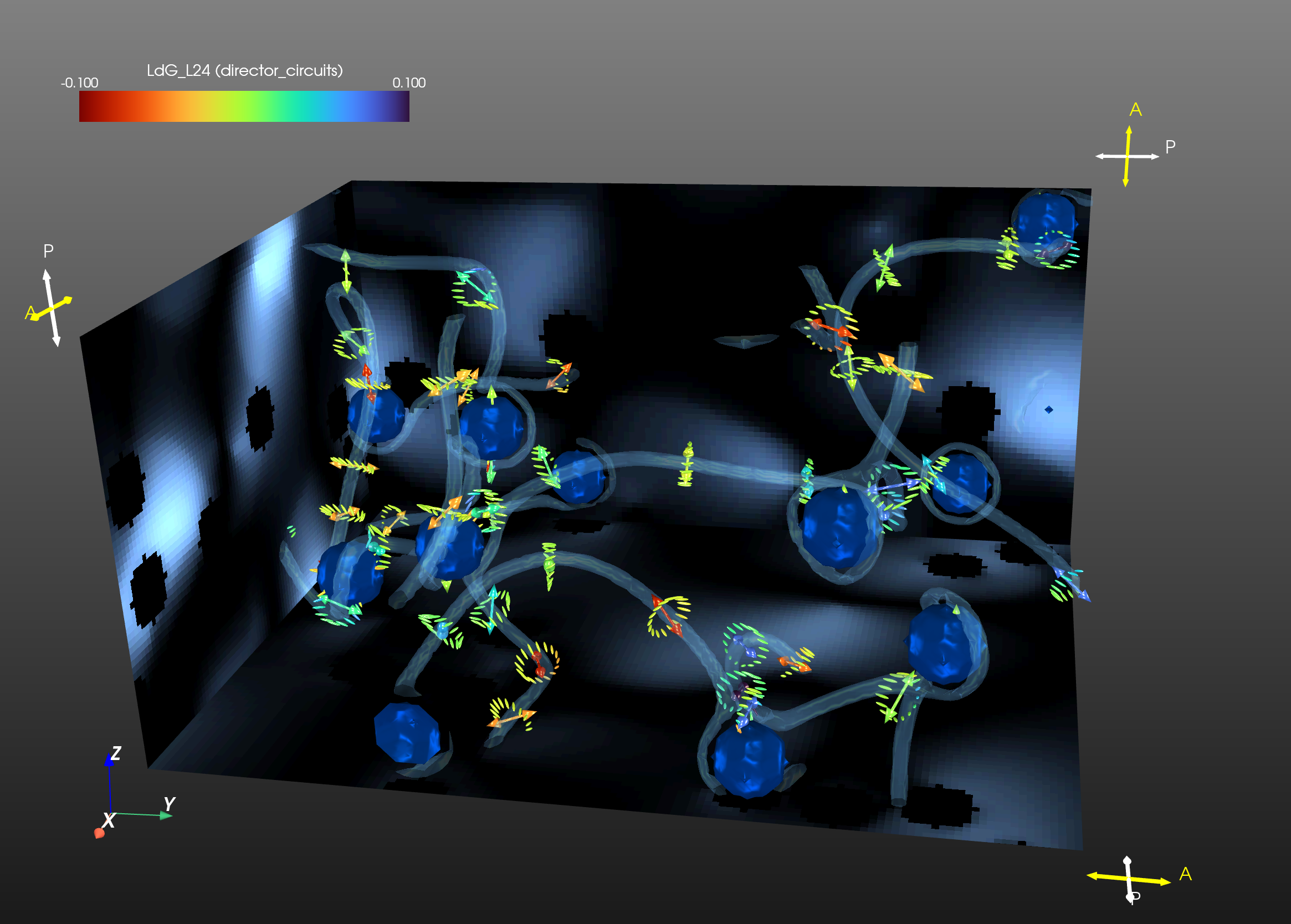
Human usin’ open-Qmin, you can zoom in!
Description#
open-ViewMin is a visualization environment for three-dimensional orientation field datasets. It is primarily designed as a visualization companion to the nematic liquid crystal modeling package open-Qmin.
The goal of open-ViewMin is to provide an environment similar to ParaView where 3D visualization is fast (ideally, GPU-accelerated) and reasonably good-looking, but that also
has a Python interface with NumPy compatibility so that users can visualize calculation results on the fly, and
comes pre-loaded with many commonly-used analysis methods for nematic LCs, such as defect identification, director slices, and Landau-de Gennes or Frank free energy components.
To do this, open-ViewMin extends PyVistaQt, a Python package that uses the Qt application-building system as the backend for PyVista, which in turn is a Python interface to the Visualization Toolkit (VTK).
In addition to details specific to nematic liquid crystals, open-ViewMin extends PyVista with FilterFormula objects, which apply PyVista filters and automatically update them when a parent mesh has changed.
Requirements#
Python 3.9, 3.10, 3.11, 3.12, or 3.13 (Unfortunately 3.14 does not work currently.)
conda or an alternative such as mamba/micromamba
Installation#
Download the source code using
git clone https://gitlab.com/open-viewmin/open-viewmin.git
cd open-viewmin
(Optional) Create a new conda environment using a Python version between 3.9 and 3.13, inclusive (we’ll use 3.11 in this example):
conda create -n "viewmin" python=3.11
conda activate viewmin
Install PyQt using conda.
conda install pyqt
If you have trouble loading open-ViewMin in iPython or Jupyter, install these in the conda environment and make the environment available to Jupyter as a kernel:
conda install ipython jupyterlab ipykernel
python -m ipykernel install --user --name=viewmin
From the
open-viewmindirectory, install open-ViewMin using pip.python -m pip install .
Basic usage#
A user can open the GUI directly from the command line as scripts/viewmin [filenames...], which calls the script at open-viewmin/scripts/viewmin.
However, more control is gained by combining the GUI and Python interfaces, so it is recommended to run the GUI in the background of a Python interpreter or Jupyter notebook.
import open_viewmin as ovm  # this might take a few minutes the first time it runs
my_plot = ovm.NematicPlot(dims=(10, 10, 10))  # empty 10x10x10 grid

# or

my_plot = ovm.NematicPlot('my_file_x0y0z0.txt')  # open-Qmin data
Treat my_plot like a dictionary in terms of accessing its meshes. To create a new mesh with a PyVista filter, use add_filter:
my_plot["sliced"] = my_plot["fullmesh"].add_filter("slice", normal=(0,0,1))
To change an existing mesh, alter the filter’s parameters using update():
my_plot["sliced"].update(normal=(1,0,0))
Change visualization options for the mesh using set():
my_plot["sliced"].set(color="green")
Terminology#
A mesh is a set of coordinates, their topology (edges and faces), and the data arrays defined on them.
This applies to point, curve, surface, and volume datasets.
A PyVista filter maps a parent mesh to a child mesh.
The child mesh inherits the parent’s data arrays.
An actor is a VTK object visualizing a mesh in the plot.
An actor is created by calling
pyvista.Plotter.add_mesh()with the mesh as the first argument.When a mesh is visualized as an actor, we give the actor the same name as the mesh.
A plotter is a window where the actors are displayed according to lighting and camera settings.
Importing data#
You can import files through the File -> Open files(s)… menu option within the GUI, or by providing the file paths as arguments when calling open-ViewMin from the command line:
viewmin file1
or
viewmin file1 file2 file3...
or from a Python interpreter or Jupyter notebook:
import open_viewmin as ovm
my_plot = ovm.NematicPlot(file1)
or
my_plot = ovm.NematicPlot([file1, file2, file3, ...])
Files from the same MPI run are assumed to be labeled as “run_name_x#y#z#.txt” (with the *#*s replaced by some integers). All such files from the same run will be combined into a single file “run_name.txt”.
Other file formats#
Some other file formats besides that of open-Qmin can be handled, but only from the Python interpreter/Jupyter notebook interface. The data_format keyword argument to NematicPlot must be specified.
If you have director data instead of Q-tensor data to import, you can import it as
import open_viewmin as ovm
my_plot = ovm.NematicPlot(
    "path/to/director_data.dat",
    data_format="director"
)
Each line of “director_data.dat” must be formatted as
x y z nx ny nz, where the first three columns contain integer coordinates and the last three contain the (float-valued) director components.For importing files from legacy-Qmin/nematicvXX, you need to provide the “Qtensor… .dat” file or files, and make sure the corresponding “Qmatrix… .dat” file is in the same folder.
import open_viewmin as ovm
my_plot = ovm.NematicPlot(
    "path/to/Qtensor_123x456x789_runname_timestep.dat",
    data_format="Qmin"
)
Usage notes for the NematicPlot GUI#
Once you’ve imported at least one file, open-ViewMin automatically creates:
a view of the director field along a slice “widget” that you can move using the mouse,
surface(s) for the boundary(ies),
isosurface of (uniaxial) nematic order to visualize defects.
Controls for these visualization elements (“actors”) will be in the right panel. For each actor, these controls include a visibility toggle checkbox and a menu of customization options.
You can add other visualizations of computed fields from the “Add” menu.
If you import more than one file, open-ViewMin will attempt to put them in order of timestamp inferred from the filenames. You can then move through the sequence of timesteps using the buttons at the top of the side toolbar area.
Non-GUI usage#
If you prefer that the GUI not open, such as if you’re generating snapshots from batch runs, use NematicPlotNoQt rather than NematicPlot:
my_plot = ovm.NematicPlotNoQt(file1)
Then, other options to visualize the results include:
save a screenshot:
my_plot.screenshot('my_image.png')render interactively in Jupyter notebook using trame backend:
my_plot.show()render interactively in Jupyter notebook using another backend, such as panel:
my_plot.extract_actors().show(jupyter_backend='panel')
In-notebook usage#
You can open an interactive view within a Jupyter notebook by creating a NematicPlotNoQt rather than a NematicPlot:
import open_viewmin as ovm
ovm.start_xvfb()
my_plot = ovm.NematicPlotNoQt(file1)
my_plot.show()
To view an existing NematicPlot within a Jupyter notebook, see Non-GUI usage above.
Computing other data arrays#
You can use Python+NumPy to compute or import data arrays other than the ones provided. This is best done in a Python interpreter or Jupyter notebook, after calling my_plot = open_viewmin.NematicPlot() from there. The plotter runs in the background, so you can execute Python commands without closing the plot.
You can view a list of the existing arrays using
my_plot['fullmesh'].array_names
You can add an array to a mesh by treating it like a Python dictionary and assigning a “key” to a NumPy array. This can be derived from existing arrays, e.g.
mesh = my_plot['fullmesh']
mesh["splay_plus_twist"] = mesh["LdG_K1"] + mesh["LdG_K2"]
or created by any other means, as long as the length of the array’s first axis equals the number of points in the mesh, e.g.
import numpy as np
my_plot['fullmesh']["my_silly_array"] = (
    np.random.random(my_plot['fullmesh'].mesh.n_points)
)
If the new array is a “scalar field” i.e. it has one value for each point in the mesh, then it will automatically appear in the appropriate submenus in the “Add” menu.
Important: In order for the new array to be inherited by the other meshes descended from “fullmesh”, you should press the Refresh button (circle of two blue arrows) in the top menu area.
License#
open-ViewMin is released open-source under the MIT license. However, open-ViewMin depends on PyVistaQt, which depends on Qt bindings to Python that have their own licenses. See https://qtdocs.pyvista.org/#license.
Roadmap#
To-do list of nematic calculations:
hedgehog charge of loop defects
chi and tau defects in cholesterics